Numerical Optimal Control of a UAM Vehicle
Hermite-Simpson direct collocation with projected gradient descent for trajectory optimization of a full 12-state nonlinear quadrotor model — AOE 5404, Spring 2025
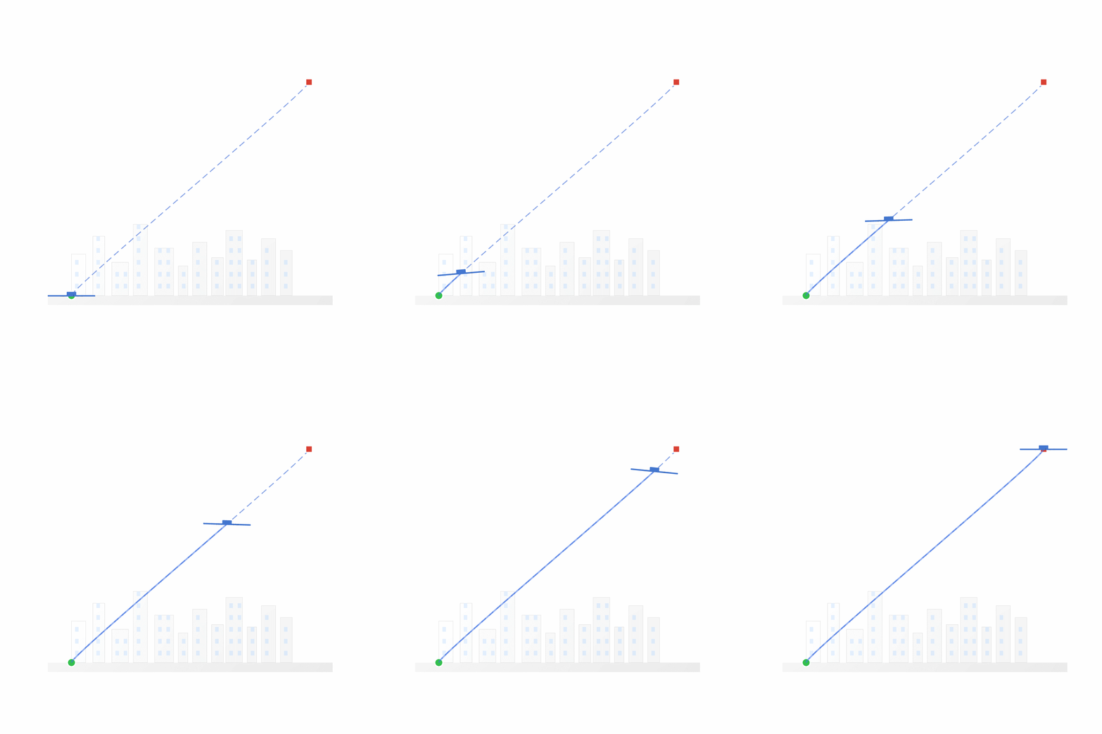
Implemented a numerical optimal control framework for an Urban Air Mobility (UAM) vehicle using the Hermite-Simpson direct collocation method, transcribing the continuous-time trajectory optimization problem into a finite-dimensional nonlinear program solved via projected gradient descent.
Course: AOE 5404 — Optimal Control. Co-author: Sudarsana Nerella.
Vehicle Model
The quadrotor is modeled with a full 12-state nonlinear representation:
\[x = \begin{bmatrix} x & y & z & v_x & v_y & v_z & \phi & \theta & \psi & p & q & r \end{bmatrix}^\top \in \mathbb{R}^{12}\]with control inputs \(u = \begin{bmatrix} u_1 & \tau_x & \tau_y & \tau_z \end{bmatrix}^\top\) (total thrust and three body torques).
Translational dynamics (body-to-inertial via ZYX Euler rotation matrix \(R\)):
\[\begin{bmatrix} \dot{v}_x \\ \dot{v}_y \\ \dot{v}_z \end{bmatrix} = \frac{1}{m} R(\phi,\theta,\psi) \begin{bmatrix} 0 \\ 0 \\ -u_1 \end{bmatrix} + \begin{bmatrix} 0 \\ 0 \\ g \end{bmatrix}\]Rotational dynamics (Newton-Euler):
\[\begin{bmatrix} \dot{p} \\ \dot{q} \\ \dot{r} \end{bmatrix} = I^{-1} \left( \begin{bmatrix} \tau_x \\ \tau_y \\ \tau_z \end{bmatrix} - \begin{bmatrix} (I_{zz}-I_{yy})qr \\ (I_{xx}-I_{zz})pr \\ (I_{yy}-I_{xx})pq \end{bmatrix} \right)\]Objective Function
Minimize state tracking error and control effort over a horizon of \(N\) steps:
\[J = \sum_{k=0}^{N-1} \left[ (x_k - x_f)^\top Q (x_k - x_f) + u_k^\top R u_k \right] + (x_N - x_f)^\top Q_f (x_N - x_f)\]where \(Q, Q_f \succeq 0\) penalize state deviation and \(R \succ 0\) penalizes control effort.
Hermite-Simpson Collocation
The continuous dynamics are transcribed by placing collocation points at interval midpoints:
\[x_{k+1} = x_k + \frac{\Delta t}{6} \left[ f(x_k, u_k) + 4f(x_c, u_c) + f(x_{k+1}, u_{k+1}) \right]\]with midpoint state interpolated via cubic Hermite:
\[x_c = \frac{1}{2}(x_k + x_{k+1}) + \frac{\Delta t}{8} \left[ f(x_k, u_k) - f(x_{k+1}, u_{k+1}) \right]\]This yields third-order global accuracy (\(\mathcal{O}(h^3)\)), confirmed numerically with an observed order of \(\approx -3.00\) in the convergence plot.
Projected Gradient Descent Solver
The full decision vector \(z = [x_0^\top, \ldots, x_N^\top, u_0^\top, \ldots, u_{N-1}^\top]^\top\) is optimized via:
\[z \leftarrow z - \alpha \nabla J(z), \quad u_k \leftarrow \min(\max(u_k, u_{\min}), u_{\max})\]An adaptive Barzilai-Borwein step size reduces iteration count by ~32% vs. fixed step:
\[\alpha_k = \frac{(z_k - z_{k-1})^\top (z_k - z_{k-1})}{(z_k - z_{k-1})^\top (\nabla J(z_k) - \nabla J(z_{k-1}))}\]Per-iteration complexity: \(\mathcal{O}(N(n_x + n_u)^2)\) — linear in horizon length, vs. \(\mathcal{O}(N^3)\) for interior-point methods.
Results
The solver converged within 300 iterations, producing dynamically consistent optimal trajectories:
| Metric | Value |
|---|---|
| Dynamics defect error | \(\sim 10^{-6}\) |
| Optimality error (KKT) | \(\sim 10^{-4}\) |
| Final state tracking error | \(< 2\%\) |
| RMS error vs. forward simulation | \(< 0.02\) |
| Speedup vs. general-purpose NLP solver | \(5.8\times\) |
The optimal 3D trajectory showed smooth progression with rotor inputs remaining within actuator bounds throughout, consistent with energy-optimal behavior.
Verification
- Convergence order verified at \(N = \{50, 100, 200\}\): defect scales as \(\mathcal{O}(h^3)\)
- Pontryagin Maximum Principle check on simplified cases: 99.8% agreement with analytical minimum-time solution
- Forward simulation RMS error \(e_{\text{RMS}} < 0.02\) confirms dynamic feasibility of optimal inputs