LQR with L1 Adaptive Augmentation — Quadrotor Trajectory Tracking
Full 6-DOF nonlinear quadrotor simulation with LQR baseline and L1 adaptive augmentation for circular trajectory tracking under Von Kármán atmospheric turbulence
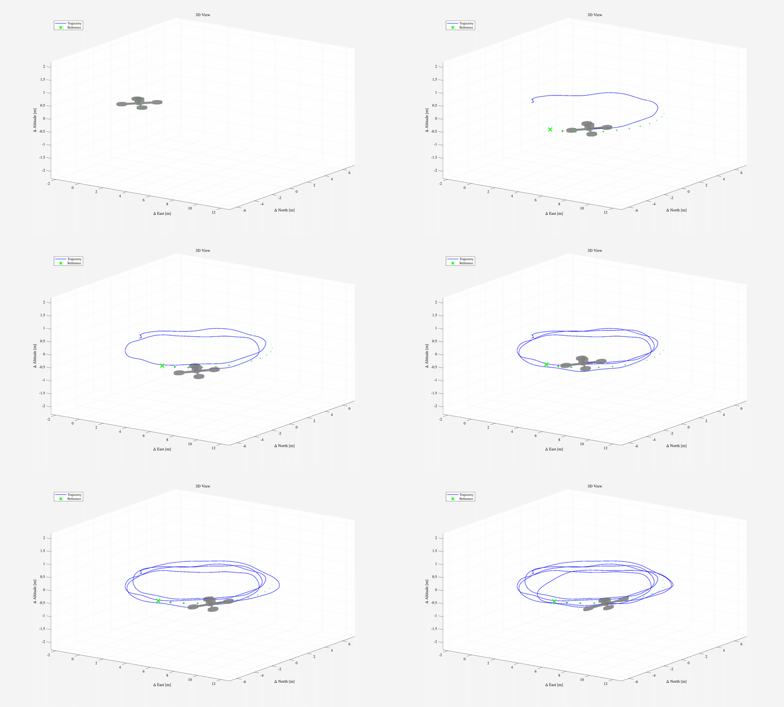
A full 6-DOF nonlinear quadrotor simulation implementing an LQR baseline controller augmented with L1 adaptive control for circular trajectory tracking under realistic atmospheric turbulence. The simulation couples rigid body dynamics, a physics-based actuator model, aerodynamic forces, and a Von Kármán turbulence field.
Vehicle Parameters
| Parameter | Value |
|---|---|
| Mass | 2.82 kg |
| Inertia \(I_{xx}\) | 0.0434 kg·m² |
| Inertia \(I_{yy}\) | 0.0453 kg·m² |
| Inertia \(I_{zz}\) | 0.0857 kg·m² |
| Arm length | 0.2030 m |
| Rotor radius | 0.1778 m |
| Number of rotors | 4 (X configuration) |
| Motor speed limits | 0 – 520 rad/s |
State and Control
The full state vector is:
\[x = \begin{bmatrix} p_N & p_E & p_D & \phi & \theta & \psi & u & v & w & p & q & r \end{bmatrix}^\top \in \mathbb{R}^{12}\]Augmented with actuator states \(\Omega \in \mathbb{R}^4\), the full 16-state system is:
\[x_a = \begin{bmatrix} x^\top & \Omega^\top \end{bmatrix}^\top \in \mathbb{R}^{16}\]Control input is commanded motor speed \(u_{\text{cmd}} \in \mathbb{R}^4\), saturated within physical limits.
Actuator Model
Each motor is modeled with first-order electrical and mechanical dynamics. The steady-state torque-speed relationship gives the equilibrium rotor speed for hover:
\[\Omega_0 : \quad F_z(\Omega_0) = -mg \implies \Omega_0 \approx 234 \text{ rad/s}\]The mixing matrix maps individual rotor thrusts to total force and moment:
\[\begin{bmatrix} T \\ \tau_x \\ \tau_y \\ \tau_z \end{bmatrix} = \underbrace{\begin{bmatrix} 1 & 1 & 1 & 1 \\ -\ell s_{45} & -\ell s_{225} & -\ell s_{315} & -\ell s_{135} \\ \ell c_{45} & \ell c_{225} & \ell c_{315} & \ell c_{135} \\ +1 & +1 & -1 & -1 \end{bmatrix}}_{\text{Mix}} \begin{bmatrix} T_1 \\ T_2 \\ T_3 \\ T_4 \end{bmatrix}\]Aerodynamic Model
The aerodynamic forces are computed using a Constant Inflow + Lumped Drag model, with 11 aerodynamic coefficients fit to the vehicle geometry. Drag is modeled as a lumped velocity-dependent force opposing body-frame motion.
Atmospheric Disturbance — Von Kármán Turbulence
Turbulence is modeled per MIL-HDBK-1797B using a Von Kármán spectral model at 200 m altitude with 10 m/s reference wind speed. The turbulence state-space model is driven by white noise:
\[\dot{x}_d = A_d x_d + B_d w(t), \quad w(t) \sim \mathcal{N}(0, I), \quad v_{\text{turb}} = C_d x_d\]A constant bulk wind component of 1 m/s North is added:
\[w_{\text{total}}(t) = \bar{w} + v_{\text{turb}}(t), \quad \bar{w} = \begin{bmatrix}1 & 0 & 0\end{bmatrix}^\top \text{ m/s}\]Reference Trajectory
Circular trajectory in the North-East plane, starting from the origin after a 5-second hover:
\[p_{\text{ref}}(t) = \begin{bmatrix} R \sin(\omega_c \tau) \\ R(1 - \cos(\omega_c \tau)) \\ 0 \end{bmatrix}, \quad \tau = \max(t - 5,\, 0)\]with radius \(R = 5\) m and angular rate \(\omega_c = 2\pi / 20\) rad/s (one lap every 20 seconds).
LQR Baseline Controller
The full 16-state system is linearized numerically at the hover trim point using complex finite difference Jacobians. The LQR gain \(K\) minimizes:
\[J = \int_0^\infty \left( \tilde{x}^\top Q \tilde{x} + \tilde{u}^\top R \tilde{u} \right) dt\]where \(\tilde{x} = x_a - [x_{\text{ref}}(t)^\top,\, \Omega_0^\top]^\top\) is the deviation from the time-varying reference.
State weights reflect physical tolerances:
| State group | Weight (1/tolerance²) |
|---|---|
| Position (N, E) | 1 m |
| Position (D) | 0.1 m |
| Euler angles (roll, pitch) | 30° |
| Yaw | 180° |
| Body velocity | 1 m/s |
| Angular rate | 30°/s |
| Motor speeds | 50 rad/s |
Control weight: \(R_u = 0.01 \cdot I_4\). Motor commands are saturated to \([0, 520]\) rad/s.
L1 Adaptive Augmentation
The L1 controller runs a state predictor in parallel with the plant at high rate, estimating and compensating matched uncertainty \(\sigma(t)\) introduced by turbulence and unmodeled aerodynamics:
\[\dot{\hat{x}} = A_m \hat{x} + B\bigl(\hat{\sigma}(t) + u_{\text{LQR}}\bigr)\]The adaptive law updates via:
\[\dot{\hat{\theta}} = -\Gamma \,\text{Proj}\!\bigl(\hat{\theta},\; \tilde{x}^\top P B\, \phi(x)\bigr), \quad \tilde{x} = \hat{x} - x\]A low-pass filter \(C(s)\) on the adaptive signal ensures bandwidth separation, bounding the \(\mathcal{L}_1\) norm and guaranteeing closed-loop robustness regardless of adaptation rate:
\[u_{\text{ad}}(s) = C(s)\,\hat{\sigma}(s), \quad \|C(s)\|_{\mathcal{L}_1} < \frac{1}{\|G(s)\|_{\mathcal{L}_1} L}\]Results
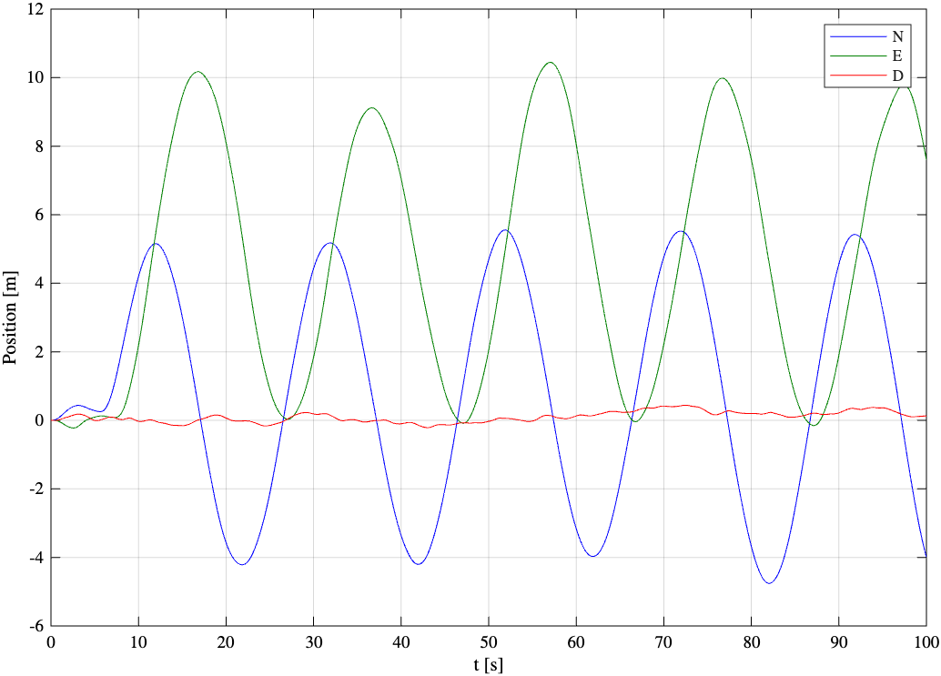
Position — North, East, Down [m]
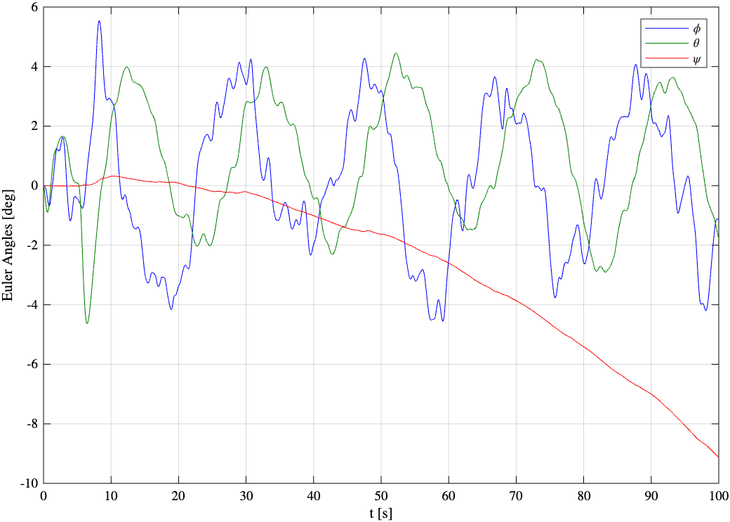
Euler Angles — roll, pitch, yaw [deg]
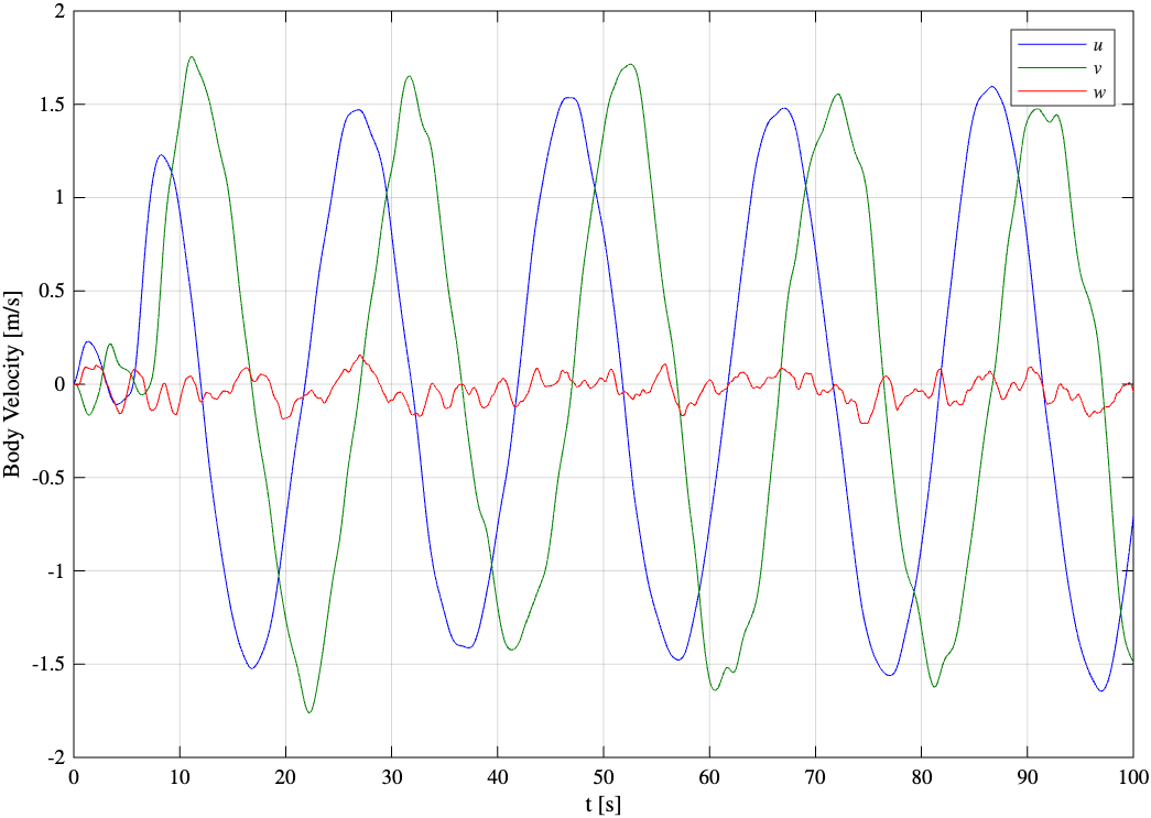
Body-frame velocity — u, v, w [m/s]
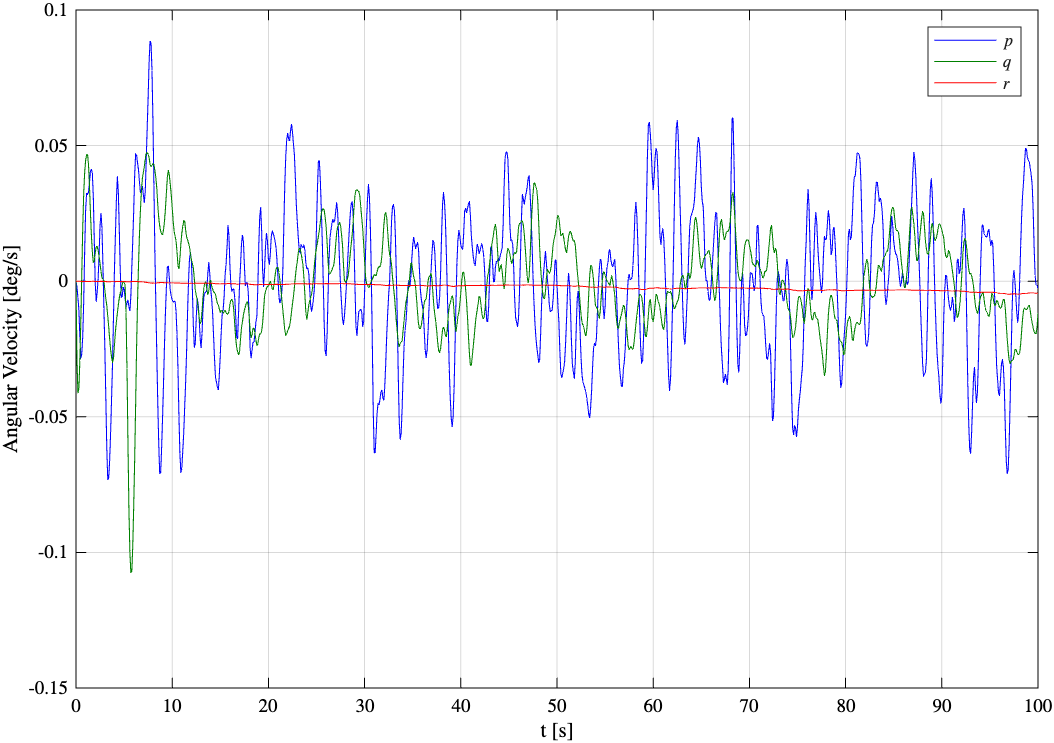
Angular velocity — p, q, r [deg/s]
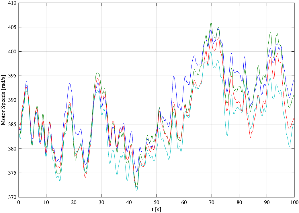
Motor speeds [rad/s]
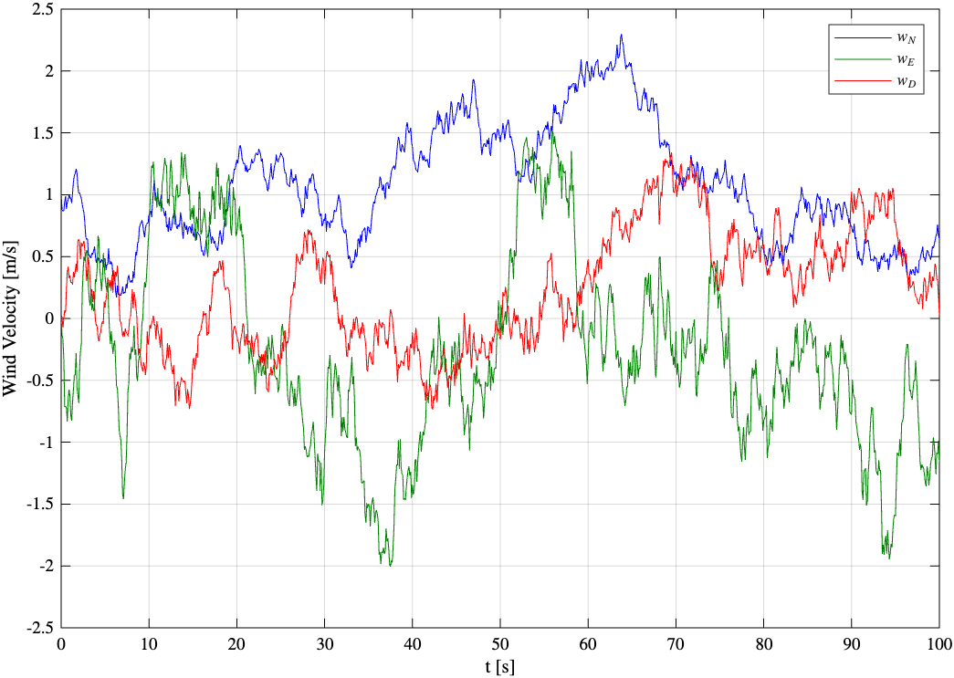
Wind velocity — North, East, Down [m/s]
Implementation
% LQR gain computed from numerically linearized hover trim
K = lqr(A, B, Q, R);

% Time-varying reference tracking with actuator saturation
u_cmd = @(t, xa) min(max( ...
    -K * (xa(1:16) - [x_ref(t); u_eq]) + u_cmd_eq, ...
    Omega_min), Omega_max);

% Augmented ODE integrating plant + actuators + turbulence states
odefun = @(t, xa) augmentedDynamics(xa, u_cmd(t,xa), wbar(t), vtil(t), ...
    aeroModel, actModel, turbModel, unstModel, params);

[ts, xa] = ode45(odefun, t, xa0, options);